Google Sheets - Get A1 Notation for Range of Named Range

If you've used Named Ranges in Google Sheets, you likely know the power of being able to refer to a range of cells with a static name without having to update the formulas in multiple cells. However, sometimes you may want to get the A1 notation (e.g. B2:C5) for that named range without looking it up in the menus.

Formula

The following formula will provide the A1 notation for a named range where named_range is the string name of a named range (without quotes):

=ADDRESS(
  ROW(
    named_range
  ),
  COLUMN(
    named_range
  ),
  4,
  TRUE
)
&":"&
ADDRESS(
  ROW(
    named_range
  )+
  ROWS(
    named_range
  )-1,
  COLUMN(
    named_range
  )+COLUMNS(
    named_range
  )-1,
  4,
  TRUE
)

Or, in one line:

'=ADDRESS(ROW(named_range),COLUMN(named_range),4,TRUE)&":"&ADDRESS(ROW(named_range)+ROWS(named_range)-1,COLUMN(named_range)+COLUMNS(named_range)-1,4,TRUE)

How it Works

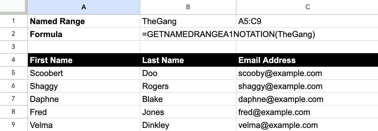
So what's happening here and how does this work? Let's assume the following simple spreadsheet:

The cells A6:C10 are defined as a named range called TheGang. For the semi-complex formula shown above, I've created a Named Function called GETNAMEDRANGEA1NOTATION() and passed in the named range as a parameter (see B4 in the screenshot above). That function returns the A1 notation for the named range TheGang, which is A7:C11.

Going back to the formula, let's break down what is happening. First, let's look at the components of the formula:

• ADDRESS(): The ADDRESS function returns a reference to the cell passed to the formula.

• ROW(): The ROW function returns the row number of a given range.

• ROWS(): The ROWS function returns the number of rows in a given range.

• COLUMN(): The COLUMN function returns the column number of a given cell.

• COLUMNS(): The COLUMNS function returns the number of columns in a given range.

Now, let's replace those functions with pseudocode to understand what is happening in the formula:

=GET_A1_NOTATION(
  NAMED_RANGE_STARTING_ROW,
  NAMED_RANGE_STARTING_COLUMN
)
&":"&
GET_A1_NOTATION(
  (NAMED_RANGE_STARTING_ROW + NAMED_RANGE_ROW_COUNT - 1),
  (NAMED_RANGE_STARTING_COLUMN + NAMED_RANGE_COLUMN_COUNT - 1
)

To simplify this formula even further, this is what is happening:

=GET_THE_A1_NOTATION_FOR_TOP_LEFT_CELL_IN_NAMED_RANGE +
":" +
GET_THE_A1_NOTATION_FOR_BOTTOM_RIGHT_CELL_IN_NAMED_RANGE

Try It Out

You can view my sample spreadsheet at the link below and you can even import the named function (`GETNAMEDRANGEA1NOTATION()` ) that I created from this sheet into your own.

Example spreadsheet with named function GETNAMEDRANGEA1NOTATION()